Control points annotation tool¶

The usage of control points during the reconstruction process in OpenSfM is documented here. This page deals with a graphical user interface to create control points manually.

The typical use case of this tool is to annotate the pixel locations surveyed ground control points on 2D images so that they can be used during the reconstruction phase for accurate georegistration.

Other less common use cases are also made possible with control points and can be realized with this tool, some of these are discussed at the end of this page:

Annotating pseudo-ground control points on orthophotos.
Annotating correspondences between two reconstructions that can’t be matched automatically. (e.g. one created during the day and another one during the night, summer-winter, and so on).
Annotating correspondences between 2D images and a 3D CAD model.

Besides annotating control points, the tool also includes features to check for correctness in the annotation by reporting and visualizing reprojection errors.

Setup¶

Install requirements:

cd OpenSfM
pip install -r annotation_gui_gcp/requirements.txt

Launch the UI on a sample dataset:

python annotation_gui_gcp/main.py data/berlin

A browser window should open. If not, visit http:/localhost:5000.

Layout¶

The tool is a multi-pane web-app. There is a main toolbox on the top and one or more panes to interact with images. The number of panes depends on the contents of the sequence_database.json file. This file defines one or more image sequences. Each sequence will open in a new window. The example dataset at data/berlin contains a single sequence in sequence_database.json

Main toolbox¶

The main toolbox contains the list of existing control points as well as several controls. The basic controls are explained here. Scroll to additional-controls for information on the rest.

The ‘Load’, ‘Save’ buttons save and load the ground control points into a ground_control_points.json file with JSON file format.
If there is a ground_control_points.json file in the dataset directory, it will be loaded upon launch.
Control points can be added or removed with the ‘Add GCP’ and ‘Remove GCP’ buttons. The active point can be selected from the dropdown.
By selecting a point in the list it becomes active and can be annotated on all images.

Image view¶

Each Image view displays a sequence of images as defined in the sequence_database.json file. The view allows navigating through the sequence and creating, deleting and correcting control points on each image. The panel on the left contains a list of frames.

Basic controls:

Clicking on a frame on the frame list will display that image.
Scrolling up/down with the mouse wheel or the up/down arrows will move to the next/previous frame.
Left clicking will create or update a control point annotation for the currently selected control point.
Right clicking will remove the control point annotation on this image.

Usage¶

Basic workflow¶

Assuming that you have a set of ground control points whose geodetic coordinates you know:

Create a OpenSfM dataset containing your images under images/ and their order in a sequence_database.json file. You can use data/berlin for this example.
Generate a ground_control_points.json file with all your measured ground control points and place it in the root of the dataset See the example below. Note how the ‘observations’ is empty as we will generate those using the annotation tool.

"points": [
  {
    "position": {"latitude": 52.519,"altitude": 14.946,"longitude": 13.400},
    "id": "my_measured_gcp_1",
    "observations": []
  }
]

Launch the annotation tool, note how the control points dropdown contains your ground control points.
Scroll through all the images, annotating each GCP on all the locations where it is visible.
Click on ‘save’ to overwrite the ground_control_points.json file with your annotations. The annotated ground control points can now be used in the OpenSfM reconstruction pipeline, see the relevant docs here.

Running the alignment and detecting wrong annotations¶

After annotating a point in more than two images, it can be triangulated using known camera poses. The reprojection of the triangulated points onto the images can be used as a check that the annotations are correct. This is enabled by the Analysis section in the main toolbox.

Ensure that there is a reconstruction.json file in the data/berlin directory. (see this link for instructions on that).
Annotate a control point in at least three images.
Save the control points using the ‘Save’ button.
Click on ‘Rigid’. After a moment, you will see output in the terminal indicating reprojection errors.

After running the analysis, the output aligned reconstructions are saved with new filenames in the root folder and can be viewed in 3D with the OpenSfM viewer.

The ‘Flex’ and ‘Full’ buttons produce additional analysis results and are explained in Aligning two reconstructions

Advanced features¶

Aligning two reconstructions¶

The tool can be used to align two reconstructions that were not reconstructed together for whatever reason (e.g. day and night or winter and summer images)

Detailed documentation for this is not available as the feature is experimental, but, in short:

Start from a dataset containing more than one reconstruction in reconstruction.json.
Launch the tool:
- If the two reconstructions come from different sequences, lauch as usual.
- If the two reconstructions come from the same sequence, launch using the --group-by-reconstruction argument. This will split the images into two windows, one for each reconstruction.
Find control points in common and annotate them. Make sure to annotate enough points to constrain the alignment.

Use the ‘Rigid’, ‘Flex’ or ‘Full’ buttons to run the alignment using the annotations:

The ‘Rigid’ option triangulates the control points in each reconstruction independently and finds a rigid transform to align them.
The ‘Flex’ option additionally re-runs bundle adjustment, allowing for some deformation of both reconstructions to fit the annotations.
The ‘Full’ option attempts to obtain positional covariances for each camera pose. If succesful, the frame list on the image views is populated with the positional covariance norm. Lower is better.

After running analysis, the reprojection errors are overlaid on the image views as shown in Running the alignment and detecting wrong annotations. The aligned reconstructions are saved with new filenames in the root folder and can be viewed in 3D with the OpenSfM viewer.

Annotating CAD models¶

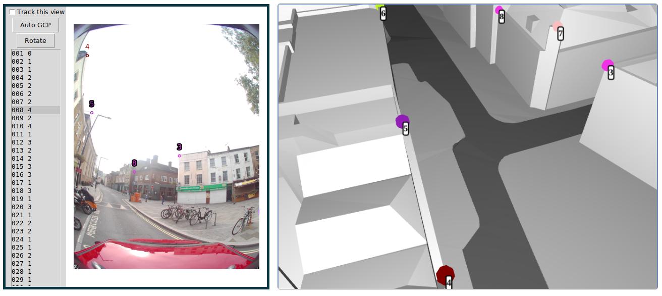
3D models in .FBX format can also be annotated with this tool.

The behavior is similar to the orthophoto annotation: the GPS coordinates of the ground-level images are used to pick from a collection of models. Annotations are 3D instead of 2D and can be used to align the SfM reconstruction with the CAD models.

This is highly experimental at the moment. Check out the –cad argument and the files in cad_viewer for more information and/or get in touch.